Experiment #3 · Mental Accounting · October 2026
Does where money comes from affect how much of it people are willing to spend?
Each participant was given the same income, the same paid time off, the same total amount of money, and the same 8-day trip to Costa Rica.
$9,667
Tax-refund mean
n = 12
+$4,108
Difference in means
Same $90,000
$5,559
Savings-only mean
n = 17
$90,000 in both groups · each block is $1,000
Savings
$80,000Checking
$10,000+$10,000 Tax Refund Deposit, last week.
Not one dollar was added or taken away. The same ten blocks either sit in savings with the rest of the salary, or move to checking with a new name. That label and that move are the only things that change.
This study examines whether the source of a person's money affects how much of it they are willing to spend, extending prior mental accounting research to an everyday online survey. Drawing on Thaler's (1985) mental accounting theory, we predicted that participants shown a $10,000 tax refund as part of their $90,000 would report a higher trip budget than those shown the same $90,000 entirely as salary savings. Twenty-nine participants were recruited via Reddit, Instagram, and my personal network and were randomly assigned to one of two conditions: a tax-refund condition ($80,000 in savings plus a $10,000 unexpected tax refund in checking) or a savings-only condition ($90,000 in savings). Each participant was given the same income, the same paid time off, the same total amount of money, and the same 8-day trip to Costa Rica. A one-tailed Welch's independent samples t-test revealed a statistically significant difference in mean trip budgets between the two groups (t = 2.488, df = 12.95, p = .0136), with the tax-refund group reporting a mean budget of $9,666.67 compared to $5,558.82 in the savings-only group. Effect size was large (Cohen's d = .999), and a 95% confidence interval for the difference in means excluded zero ($539.97, $7,675.73), consistent with the result. These findings are consistent with mental accounting and prior work by Arkes et al. (1994), suggesting that money which arrives unexpectedly is spent more readily than money that was earned and saved, even when the total is identical. Limitations of this study, including small sample size, convenience sampling, a skewed tax-refund group, and a possible anchoring confound, are discussed alongside directions for future research.
In theory, money is fungible. A dollar from a paycheck and a dollar from a tax refund buy the exact same things, so where a dollar came from shouldn't change how it gets spent. In practice, people rarely treat money this way. Instead, the mind sorts money into separate mental "accounts" based on where it came from and where it sits, and each account gets its own spending rules. This is mental accounting, formally developed by Richard Thaler in 1985. Simply put, your brain guards the money it worked for, and treats money that showed up unexpectedly as free to spend.
Research question
Does where money comes from affect how much of it people are willing to spend?
Hypothesis
Respondents shown a $10,000 tax refund as part of their $90,000 will report a higher trip budget, on average, than those shown the same $90,000 entirely as salary savings, consistent with Thaler's (1985) mental accounting theory.
H₀ Null
There is no difference in mean trip budgets between the tax-refund and savings-only groups. μ₁ = μ₂
H₁ Alternative
Mean trip budget will be higher for the tax-refund group than the savings-only group. μ₁ > μ₂
Participants were given a hypothetical situation of planning an 8-day, 7-night trip to Costa Rica and were shown a snapshot of their finances. In both groups the total amount of money was $90,000, the monthly take-home pay was $9,000, and there were 12 PTO days remaining, but the money was split across accounts differently.
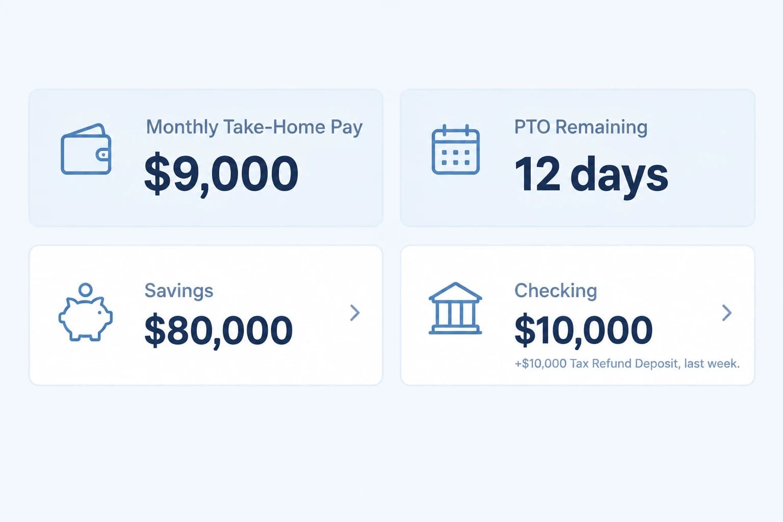
Group 1 saw this text:
You are 26 years old, unmarried, and work full-time. You net $9000 every month after expenses, and your savings account consists entirely of your own salary saved up. You recently got a huge, unexpected tax refund worth $10,000, which deposited straight into your checkings account. Your 12 PTO (Paid time off) days expire on December 31 and do not roll over, so you wish to use them soon. You're going on an 8-day, 7-night trip to Costa Rica. What is your budget for this trip, in USD? What are you willing to spend out of your accounts to make this trip memorable yet financially feasible?
Everything outside the highlight is identical, character for character, in both conditions.
Your budget
Closest level: Regular (~$6,000)
$6,000
Randomizer validation · n = 10,000
A 49.81 / 50.19 split across ten thousand trials. The same randomizer then sent 12 real participants one way and 17 the other.
How treatment assignment worked
G1
Tax refund
Group shown the $10,000 tax refund ($80,000 savings + $10,000 checking) · n = 12
G2
Savings only
Group shown savings only ($90,000 savings) · n = 17
Every budget chart below shares one dollar axis, with the four levels from the budget graphic marked along it, so you can see which level each answer landed nearest.
Descriptive statistics
| G1$10,000 tax refund | G2Savings only | |
|---|---|---|
| Mean | $9,666.67 | $5,558.82 |
| Median | $7,500 | $6,000 |
| Standard deviation | $5,482.76 | $1,935.54 |
| Range | $17,000 | $7,000 |
| IQR | $6,500 | $2,500 |
| n | 12 | 17 |
| Outliers | None | 1 outlier, value $10,000 |
Outliers using the 1.5x IQR rule.
Means and medians · boxes span the IQR
The means sit $4,107.85 apart. Switch to medians to see how much of that survives.
Name: one-tailed Welch's independent samples t-test
Alpha level: .05Conditions
Click each to check.
Distribution of responses
G1 stacks above the axis, G2 below. Dotted guides mark the four budget levels; dashed verticals mark each group mean; the dashed ring is G2's outlier.
Before you scroll. Means $4,107.85 apart, medians only $1,500 apart, 12 against 17 people. Was that significant at α = 0.05?
Practicality · Cohen's d
0.999
To assess the practical significance of the result, Cohen's d was calculated using the means and standard deviations of both groups. Cohen's d = 0.999 using average variance formula (unpooled), which indicates a largeeffect by Cohen's (1988) conventions (small = 0.2, medium = 0.5, large = 0.8). This suggests that the difference in trip budgets between the two groups was not only statistically significant but also practically meaningful. One caution is that the medians ($7,500 vs $6,000) are only $1,500 apart, so a large part of the $4,107.85 gap in means comes from a few very high budgets in G1.
95% confidence interval · difference in means (G1 − G2)
A 95% confidence interval for the difference in mean trip budgets (G1 - G2) was calculated as ($539.97, $7,675.73). This means we are 95% confident that the true difference in mean trip budgets between the tax-refund and savings-only groups falls between $539.97 and $7,675.73. 0 not being included within our interval is consistent with our decision to reject the null hypothesis. The interval is wide, which reflects how small the sample is.
My findings support the hypothesis. The group shown the tax refund reported a mean trip budget of $9,666.67, while the group shown savings only reported a mean trip budget of $5,558.82. Both groups had the exact same $90,000, the same income, and the same trip, yet we found significant evidence that people budgeted more when part of that money was shown as an unexpected refund. The tax-refund group's mean budget also landed almost exactly on the size of the refund itself.
The real-world implications span a lot of domains
Each card shows only the label money wears. Click for the rest.
These are all examples where money gets treated differently because of its label, not its value. These are mental accounting in action.
I changed two things at once. In G1, $10,000 was labeled as an unexpected tax refund and it was also moved from savings to checking. Both are mental accounting manipulations, but I can't separate how much of the effect came from the source of the money versus the account it sat in.
Anchoring is a competing explanation. G1 saw the number $10,000 three times outside of the budget graphic (in the text, as the checking balance, and in the deposit note), while G2 never did. G1's mean of $9,666.67 landing that close to $10,000 could partly be an anchor on that number rather than mental accounting.
G1 was small (n = 12) and right-skewed. The medians were only $1,500 apart, so the gap in means was driven by a few very high budgets, and the normality condition was only weakly met. The p value is less trustworthy than it looks.
Because my Instagram account is framed as a behavioral economics account, and I posted in r/behavioraleconomics along with more general subreddits like r/samplesize and r/surveyexchange, some participants likely went into the survey already expecting some kind of psychological trick.
If anyone took the survey twice and saw both treatments, it could contaminate responses.
Times each group saw “$10,000” outside the budget graphic
$10,000
The refund
$9,666.67
G1 mean
~$10,000
Luxury level
Ways this experiment could be improved are as follows.
My sample size needs to be substantially larger, ideally upwards of 100 participants per group to improve statistical power and allow for more reliable replication.
I would separate the two things I changed at once by running four groups (refund in checking, refund in savings, salary in checking, and salary in savings) to see whether the label or the location drives the effect.
I would also use a refund amount that doesn't match any number on the budget graphic, like $8,500, or remove the graphic entirely, to rule out anchoring.
Other directions include testing whether the size of the windfall matters ($1,000 vs $10,000 vs $50,000), comparing the tax refund against other sources of unexpected money like a bonus, a gift, or lottery winnings, asking participants to state their total money before giving a budget to see if making the full $90,000 obvious weakens the effect, and running a Mann-Whitney U test alongside the t-test, since budget data tends to be skewed.
The four groups, and the two this study ran
G1 · this study
n = 12
Not yet run
Not yet run
G2 · this study
n = 17
This study ran only the diagonal, so the name on the money and the account it sat in always moved together. The two empty cells are what would pull them apart.
Experiment #3 · October 2026